
Quantum sensing for robot navigation#
A robot that loses GPS has to navigate by integrating its accelerometer twice, and any bias in the accelerometer becomes a position error that grows with time. A cold-atom interferometer is a quantum sensor with very small noise and almost no drift, but it is slow. This tutorial derives its quantum-limited sensitivity, then asks in simulation what fusing it with a fast, drifting MEMS accelerometer does to a robot’s position estimate, and when it does not help. Sensor values are illustrative assumptions and the trajectory is simulated.
import numpy as np
import matplotlib.pyplot as plt
from quantum_mind.viz import use_mpl_style
from quantum_mind.sensing import (phase_sensitivity, atom_interferometer_sensitivity, mems_accelerometer,
                                  atom_interferometer_accelerometer, compare_sensor_suites, simulate_dead_reckoning, run_filter)
theme = use_mpl_style('dark')
1. The quantum limit#
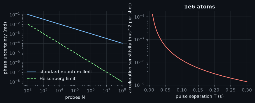
A phase read from N probes is limited by the standard quantum limit 1/sqrt(N); entangled probes can in principle reach
1/N (the Heisenberg limit). An atom interferometer turns acceleration into phase, phi = k_eff a T^2, so its acceleration
sensitivity improves with the atom number and, quickly, with the pulse separation T.
N = np.logspace(2, 8, 50)
T = np.linspace(0.01, 0.3, 50)
fig, ax = plt.subplots(1, 2, figsize=(9.2, 3.0))
ax[0].loglog(N, [phase_sensitivity(n) for n in N], color=theme['palette'][1], label='standard quantum limit')
ax[0].loglog(N, [phase_sensitivity(n, scaling='heisenberg') for n in N], color=theme['palette'][3], ls='--', label='Heisenberg limit')
ax[0].set_xlabel('probes N'); ax[0].set_ylabel('phase uncertainty (rad)'); ax[0].legend(frameon=False)
ax[1].semilogy(T, [atom_interferometer_sensitivity(1e6, t) for t in T], color=theme['palette'][0])
ax[1].set_xlabel('pulse separation T (s)'); ax[1].set_ylabel('acceleration sensitivity (m/s^2 per shot)')
ax[1].set_title('1e6 atoms')
plt.show()
mems, quantum = mems_accelerometer(), atom_interferometer_accelerometer()
print('per-sample noise: MEMS %.1e m/s^2 at %g Hz, atom interferometer %.1e m/s^2 at %g Hz'
      % (mems.noise_std, mems.rate_hz, quantum.noise_std, quantum.rate_hz))
per-sample noise: MEMS 9.8e-03 m/s^2 at 100 Hz, atom interferometer 1.2e-08 m/s^2 at 1 Hz
2. Dead reckoning with one sensor or both#
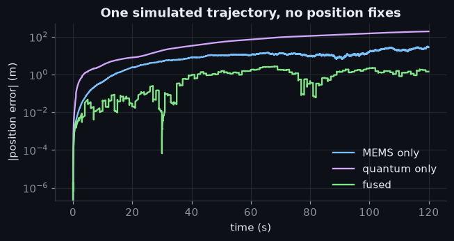
A one-axis robot with an unknown acceleration. A multi-rate Kalman filter estimates position, velocity, acceleration and each sensor’s bias. Without any outside reference the MEMS sensor drifts; the quantum sensor alone is stable but too slow to follow the acceleration; together, the quantum sensor lets the filter see the MEMS bias.
data = simulate_dead_reckoning([mems, quantum], duration=120, seed=2)
t = np.arange(len(data.pos)) * data.dt
fig, ax = plt.subplots(figsize=(6.6, 3.0))
for label, names, c in (('MEMS only', [mems.name], 1), ('quantum only', [quantum.name], 2), ('fused', [mems.name, quantum.name], 3)):
    ax.plot(t, np.abs(run_filter(data, names)), label=label, color=theme['palette'][c])
ax.set_yscale('log'); ax.set_xlabel('time (s)'); ax.set_ylabel('|position error| (m)'); ax.legend(frameon=False)
ax.set_title('One simulated trajectory, no position fixes')
plt.show()
suites = {'MEMS only': [mems.name], 'quantum only': [quantum.name], 'fused': [mems.name, quantum.name]}
rows = compare_sensor_suites([mems, quantum], suites, duration=120, seeds=range(4))
for r in rows:
    print('%-13s RMSE %.2f +- %.2f m' % ((r['suite'],) + r['rmse']))
MEMS only     RMSE 47.93 +- 28.71 m
quantum only  RMSE 44.47 +- 34.34 m
fused         RMSE 1.93 +- 1.10 m
3. When the quantum sensor does not help#
The benefit comes from the quantum sensor being stable. Make its bias as large as the MEMS bias (its white noise stays at the quantum limit) and the benefit goes away. A position fix every 10 s also removes most of the problem for the MEMS sensor alone.
ratios = {}
for frac in (1e-4, 1e-2, 1.0):
    q = atom_interferometer_accelerometer(bias_walk=frac * mems.bias_walk, bias_std0=frac * mems.bias_std0)
    res = compare_sensor_suites([mems, q], {'mems': [mems.name], 'fused': [mems.name, q.name]}, duration=120, seeds=range(4))
    ratios[frac] = res[1]['rmse'][0] / res[0]['rmse'][0]
    print('quantum bias = %g x MEMS bias: fused / MEMS-only RMSE = %.3f' % (frac, ratios[frac]))
fixed = compare_sensor_suites([mems, quantum], suites, duration=120, seeds=range(4), fix_period=10.0)
print({r['suite']: round(r['rmse'][0], 3) for r in fixed})
quantum bias = 0.0001 x MEMS bias: fused / MEMS-only RMSE = 0.040
quantum bias = 0.01 x MEMS bias: fused / MEMS-only RMSE = 0.034
quantum bias = 1 x MEMS bias: fused / MEMS-only RMSE = 0.455
{'MEMS only': 0.179, 'quantum only': 1.77, 'fused': 0.132}
The statements below are checked by this cell every time the documentation is built:
assert phase_sensitivity(100, scaling='heisenberg') < phase_sensitivity(100)
assert atom_interferometer_sensitivity(1e6, 0.2) < atom_interferometer_sensitivity(1e6, 0.1) / 3
assert rows[2]['rmse'][0] < rows[0]['rmse'][0] / 3                      # fusing beats MEMS alone by a wide margin
assert rows[2]['rmse'][0] < rows[1]['rmse'][0]                           # and the slow quantum sensor alone
assert ratios[1e-4] < 0.2 < ratios[1.0]                                  # the benefit disappears as the quantum bias grows
assert fixed[0]['rmse'][0] < rows[0]['rmse'][0] / 20                     # position fixes alone remove most of the MEMS drift
print('checked')
checked
Summary. In this simulation a quantum accelerometer helps a drifting MEMS sensor a great deal when there is no outside
reference, because its stability lets the filter calibrate the MEMS bias, even though it is far too slow to navigate alone. The
benefit shrinks as the quantum sensor’s own bias grows, and an occasional position fix makes the MEMS sensor good enough on its
own. The sensor numbers are assumptions; a real instrument has to be measured. benchmarks/quantum_sensing_benchmark.py runs
the full study with paired tests.
References: Kasevich & Chu (1992), Applied Physics B 54, 321; Giovannetti, Lloyd & Maccone (2004), Science 306, 1330; Kalman (1960), Journal of Basic Engineering 82, 35.