Quantum computing for robot algorithms#

A team of robots has to decide who does which task. That is a combinatorial optimisation problem, the kind that quantum algorithms such as QAOA are proposed for. This tutorial encodes robot problems as QUBOs, solves them with classical solvers and with QAOA (Qiskit’s QAOAAnsatz on an exact simulator, not hardware), and asks the question that matters: does the quantum solver beat the classical baselines, including random guessing with the same number of samples? The data are simulated.

import warnings
import numpy as np
import matplotlib.pyplot as plt
from quantum_mind.viz import use_mpl_style
from quantum_mind.computing import (multi_robot_allocation, grasp_selection, slot_scheduling, compare_solvers,
                                    greedy_descent, simulated_annealing, random_sampling, qaoa)
warnings.simplefilter('ignore')
theme = use_mpl_style('dark')

1. A robot problem and its encoding#

Three robots, three tasks, a cost for each pair. The QUBO has one binary variable per robot-task pair and a penalty that forces every task onto exactly one robot. RobotProblem also keeps the true objective (the total cost, without the penalty), so an answer is judged on the robot’s terms.

rng = np.random.default_rng(3)
costs = rng.uniform(1, 9, (3, 3))
problem = multi_robot_allocation(costs, balance=0.3)
x_opt, value = problem.optimum()
print('variables:', problem.n_variables, '| optimum:', problem.decode(x_opt), 'objective %.3f' % value)

variables: 9 | optimum: {0: [0], 1: [2], 2: [1]} objective 9.328

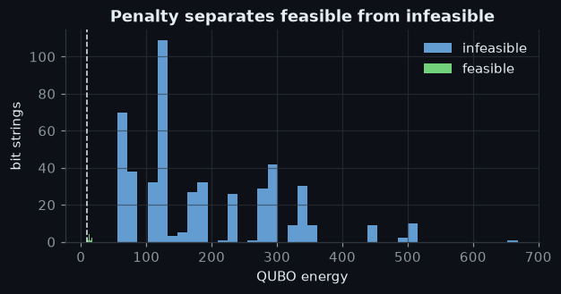
The minimiser of the QUBO is the true optimum, and every infeasible bit string has a higher energy:

energies = problem.qubo.all_energies()
n = problem.n_variables
X = (np.arange(2 ** n)[:, None] >> np.arange(n)) & 1
feasible = np.array([problem.feasible(r) for r in X])
print('feasible strings: %d of %d | best infeasible energy %.2f > optimum energy %.2f'
      % (feasible.sum(), 2 ** n, energies[~feasible].min(), energies.min()))
fig, ax = plt.subplots(figsize=(6.2, 2.8))
ax.hist(energies[~feasible], bins=40, color=theme['palette'][1], alpha=0.8, label='infeasible')
ax.hist(energies[feasible], bins=10, color=theme['palette'][3], alpha=0.9, label='feasible')
ax.axvline(energies.min(), color=theme['text'], ls='--', lw=1)
ax.set_xlabel('QUBO energy'); ax.set_ylabel('bit strings'); ax.set_title('Penalty separates feasible from infeasible'); ax.legend(frameon=False)
plt.show()

feasible strings: 27 of 512 | best infeasible energy 55.90 > optimum energy 9.33

Figure: Penalty separates feasible from infeasible

2. The same problem, several solvers#

compare_solvers runs exhaustive search (the optimum), greedy descent, simulated annealing, random sampling with the same 1000 shots and QAOA at depth 2, and reports each in robot terms.

rows = compare_solvers(problem, seed=1)
for r in rows:
    print('%-24s feasible %-5s gap %s' % (r['solver'], r['feasible'], 'n/a' if r['gap'] is None else '%.3f' % r['gap']))
qaoa_row = next(r for r in rows if r['solver'].startswith('QAOA'))
print('QAOA: P(optimal) = %.4f, uniform guess = %.4f' % (qaoa_row['info']['p_optimal'], 2.0 ** -n))

exhaustive               feasible True  gap 0.000
simulated annealing      feasible True  gap 0.075
greedy descent           feasible True  gap 0.000
random sampling (1000)   feasible True  gap 0.000
QAOA (Qiskit, p=2)       feasible True  gap 0.000
QAOA: P(optimal) = 0.0012, uniform guess = 0.0020

3. Is QAOA better than guessing?#

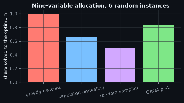
A sampling solver that returns the best of 1000 samples looks good on a problem with only 512 bit strings simply because it draws so many. The honest comparison is the share of instances each solver solves to the exact optimum, over several random problems.

rng = np.random.default_rng(11)
solved = {k: 0 for k in ('greedy descent', 'simulated annealing', 'random sampling', 'QAOA p=2')}
p_opt, n_inst = [], 6
for _ in range(n_inst):
    p = multi_robot_allocation(rng.uniform(1, 9, (3, 3)), balance=0.3)
    opt = p.optimum()[1]
    res = {'greedy descent': greedy_descent(p.qubo, restarts=20, seed=1),
           'simulated annealing': simulated_annealing(p.qubo, seed=1),
           'random sampling': random_sampling(p.qubo, 1000, seed=1),
           'QAOA p=2': qaoa(p.qubo, depth=2, restarts=2, maxiter=100, seed=1)}
    for k, r in res.items():
        solved[k] += bool(p.feasible(r.x) and abs(p.objective(r.x) - opt) < 1e-9)
    p_opt.append(res['QAOA p=2'].info['p_optimal'])
print({k: '%d/%d' % (v, n_inst) for k, v in solved.items()})
print('QAOA mean probability on the optimum: %.4f (uniform guess %.4f)' % (np.mean(p_opt), 2.0 ** -n))
fig, ax = plt.subplots(figsize=(6.2, 2.8))
ax.bar(list(solved), [v / n_inst for v in solved.values()], color=theme['palette'][:4])
ax.set_ylim(0, 1.05); ax.set_ylabel('share solved to the optimum'); ax.set_title('Nine-variable allocation, %d random instances' % n_inst)
plt.setp(ax.get_xticklabels(), rotation=12)
plt.show()

{'greedy descent': '6/6', 'simulated annealing': '4/6', 'random sampling': '3/6', 'QAOA p=2': '5/6'}
QAOA mean probability on the optimum: 0.0038 (uniform guess 0.0020)

Figure: 3. Is QAOA better than guessing?

The statements below are checked by this cell every time the documentation is built:

assert problem.feasible(x_opt) and np.isclose(problem.objective(x_opt), value)
assert energies[~feasible].min() > energies.min()                       # the penalty works
assert abs(rows[0]['gap']) < 1e-9                                        # exhaustive search is exact
assert solved['greedy descent'] == n_inst                                # a simple classical baseline solves all of them
assert np.mean(p_opt) < 0.2                                              # QAOA puts a small share on the optimum
assert qaoa_row['feasible'] and 0 <= qaoa_row['info']['p_optimal'] <= 1  # and returns a valid, feasible answer
print('checked')

checked

Summary. On problems small enough to enumerate, greedy descent solves every instance, random sampling with the same shots solves a large share of them, and QAOA at depth 2 puts only a small probability on the optimum, of the order of a uniform guess for this problem (compare the two numbers printed above; the exact counts depend on the random instances). That does not say what happens on problems too large to enumerate or on quantum hardware; it says that “QAOA solved my robot problem” means little unless the classical baselines and the random-sampling null were run next to it. benchmarks/robot_quantum_computing_benchmark.py repeats this for three problems and three QAOA depths.

References: Lucas (2014), Frontiers in Physics 2, 5; Farhi, Goldstone & Gutmann (2014), arXiv:1411.4028.