Introduction to Quantum Mind#

This first tutorial shows the three ideas that everything else in the library builds on:

a belief is a unit vector, and a question is a projector;
answering a question changes the belief (Lüders’ rule), so the order of questions can matter;
every model is fitted to data and compared with classical models on the same data.

It then points to where each pillar of the library lives. Run it top to bottom; it takes a few seconds.

import numpy as np
import matplotlib.pyplot as plt
import quantum_mind
from quantum_mind.viz import use_mpl_style
theme = use_mpl_style('dark')          # the colours of the docs and the Bloch-sphere viewer
print('Quantum Mind', quantum_mind.__version__)

Quantum Mind 3.1.0

1. A belief and two questions#

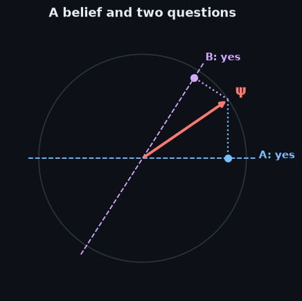
A person’s belief about a topic is a unit vector \(\psi\) in a small real space. A yes/no question is a projector \(P\) onto the “yes” subspace, and the probability of “yes” is \(\|P\psi\|^2\) (the Born rule). Here the space is two-dimensional, so each “yes” subspace is a line at some angle.

from quantum_mind.core.linalg import normalize, projector, luders

psi = normalize(np.array([np.cos(0.6), np.sin(0.6)]))      # the belief, 0.6 rad from the x axis
a, b = 0.0, 1.0                                              # angles of the two "yes" directions
PA = projector([[np.cos(a), np.sin(a)]])
PB = projector([[np.cos(b), np.sin(b)]])

p_yes_A = np.linalg.norm(PA @ psi) ** 2
p_yes_B = np.linalg.norm(PB @ psi) ** 2
print('P(yes to A) = %.3f   P(yes to B) = %.3f' % (p_yes_A, p_yes_B))

P(yes to A) = 0.681   P(yes to B) = 0.848

2. Answering changes the belief, so order matters#

After a “yes” to A, the belief collapses onto the A direction (Lüders’ rule). The chance of then saying “yes” to B is computed from the new belief. Doing it in the other order gives a different joint probability, because \(P_A\) and \(P_B\) do not commute.

def p_yes_yes(first, second, psi):
    p1, after = luders(psi, first)                             # P(yes) and the belief after "yes"
    p2, _ = luders(after, second)
    return p1 * p2

print('P(yes A, then yes B) = %.3f' % p_yes_yes(PA, PB, psi))
print('P(yes B, then yes A) = %.3f' % p_yes_yes(PB, PA, psi))
print('commute?', np.allclose(PA @ PB, PB @ PA))

P(yes A, then yes B) = 0.199
P(yes B, then yes A) = 0.248
commute? False

The picture: the belief (coral), the two “yes” directions and the projections onto them.

fig, ax = plt.subplots(figsize=(4.6, 4.6))
t = np.linspace(0, 2 * np.pi, 200)
ax.plot(np.cos(t), np.sin(t), color=theme['wire'], lw=1)
for ang, name, c in ((a, 'A: yes', theme['palette'][1]), (b, 'B: yes', theme['palette'][2])):
    ax.plot([-1.1 * np.cos(ang), 1.1 * np.cos(ang)], [-1.1 * np.sin(ang), 1.1 * np.sin(ang)], '--', color=c, lw=1.2)
    ax.text(1.12 * np.cos(ang), 1.12 * np.sin(ang), name, color=c, fontweight='bold')
ax.annotate('', xy=psi, xytext=(0, 0), arrowprops=dict(arrowstyle='-|>', color=theme['palette'][0], lw=2.5))
for P, c in ((PA, theme['palette'][1]), (PB, theme['palette'][2])):
    proj = P @ psi
    ax.plot([psi[0], proj[0]], [psi[1], proj[1]], ':', color=c)
    ax.scatter(*proj, color=c, s=40, zorder=3)
ax.text(*(psi * 1.08), 'ψ', color=theme['palette'][0], fontsize=14, fontweight='bold')
ax.set_aspect('equal'); ax.set_xlim(-1.3, 1.3); ax.set_ylim(-1.3, 1.3); ax.grid(False)
ax.set_title('A belief and two questions'); ax.axis('off')
plt.show()

3. Fit and compare, always against classical models#

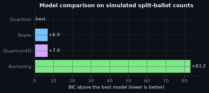
Real data are counts of answers in each order. Here the counts are simulated from a quantum-like model (500 people per order), then four models are fitted and compared by BIC (lower is better). The Bayesian model has no order effect, so it should lose; the anchoring model is the classical model that does allow order effects.

from quantum_mind.core import compare
from quantum_mind.families.order_effects import (QuantumOrderModel, QuantumOrderModel4D, AnchoringOrderModel,
                                                 BayesOrderModel, RANK_STRUCTURES, qq_test)

truth = QuantumOrderModel(a=2.35, b=0.97, g=0.58, ranks=(1, 2))
counts = truth.sample(None, 500, np.random.default_rng(1))
print('simulated counts (yes-yes, yes-no, no-yes, no-no):', {k: v.tolist() for k, v in counts.items()})

results = compare([QuantumOrderModel4D, (QuantumOrderModel, {'structures': RANK_STRUCTURES}),
                   AnchoringOrderModel, BayesOrderModel], counts, restarts=8)
for r in results:
    print('  %-22s BIC %7.1f' % (type(r.model).__name__, r.bic))
q, z, p = qq_test(counts)
print('QQ test (projective models predict q = 0): q = %.3f, p = %.3f' % (q, p))

simulated counts (yes-yes, yes-no, no-yes, no-no): {'AB': [241, 1, 71, 187], 'BA': [290, 57, 0, 153]}

  QuantumOrderModel      BIC  1959.7
  BayesOrderModel        BIC  1966.6
  QuantumOrderModel4D    BIC  1966.7
  AnchoringOrderModel    BIC  2042.9

QQ test (projective models predict q = 0): q = 0.030, p = 0.157

names = [type(r.model).__name__.replace('OrderModel', '') for r in results]
bics = np.array([r.bic for r in results])
fig, ax = plt.subplots(figsize=(6.4, 2.6))
gap = bics - bics.min()
ax.barh(names[::-1], gap[::-1], color=theme['palette'][:len(names)][::-1])
for i, g in enumerate(gap[::-1]):
    ax.text(g + 0.5, i, 'best' if g == 0 else '+%.1f' % g, va='center', color=theme['text'])
ax.set_xlabel('BIC above the best model (lower is better)')
ax.set_title('Model comparison on simulated split-ballot counts')
plt.show()

Figure: Model comparison on simulated split-ballot counts

4. The rest of the library#

Pillar	What it holds	Start with
Quantum-like	four families of models of order effects, inference, trust and perception	tutorials 2, 3, 9
Robot decision layer	ask or act, calibration, orchestration, question planning, fusion, hand-over	tutorials 4 to 8
COBRA belief filter	a density-matrix belief whose measurement basis is rotated by the previous sensor frame	tutorial 10
Viewer	Bloch spheres, trajectories and animations	tutorial 11

Every model also has a block diagram in the model atlas, and the foundations pages explain the background from the basics.