
Choosing between perception modules#
A robot often has several modules that can answer the same question: a fast on-board detector, a larger model on a GPU, a cloud vision-language model, or asking a person. Each has a cost and a confidence. The confidence gate picks the module with the best confidence-minus-cost trade-off, and can stay within a budget. But raw confidences are biased differently for each module, and a new task starts with no data about those biases. The meta-calibrated gate learns, from earlier tasks, how biased each module usually is, and uses that as a prior on a new task.
Everything here is simulated: tasks draw a hidden confidence bias per module.
import numpy as np
import matplotlib.pyplot as plt
from quantum_mind.viz import use_mpl_style
from quantum_mind.applications.orchestration import (Module, ConfidenceGate, MetaCalibratedGate, RoutingTask,
                                                     simulate_routing, meta_fit_offsets)
theme = use_mpl_style('dark')
print('module costs:', RoutingTask.COST, '  mean confidence bias per module:', RoutingTask.MEAN_OFFSETS)
module costs: (1.0, 3.0, 2.0, 4.0) mean confidence bias per module: (0.0, 0.3, 0.25, 0.05)
1. The cost-penalised gate#
The gate scores each module as confidence - lam × cost and picks the best. A larger lam makes the
robot thriftier.
mods = [Module('on-board', 1.0), Module('GPU model', 3.0), Module('cloud VLM', 4.0)]
conf = [0.70, 0.86, 0.93]
for lam in (0.0, 0.03, 0.1):
    k = ConfidenceGate(mods, lam=lam).select(conf)
    print('lam = %.2f -> %s' % (lam, mods[k].name))
lam = 0.00 -> cloud VLM
lam = 0.03 -> cloud VLM
lam = 0.10 -> on-board
2. Learn the biases from earlier tasks#
Log 30 earlier tasks (random module choices, observed successes) and fit the average bias of each module and how much it varies between tasks (an empirical-Bayes prior).
rng = np.random.default_rng(0)
logs = []
for _ in range(30):
    task = RoutingTask.sample(rng)
    log = []
    for _ in range(300):
        p, c = task.step(rng)
        k = int(rng.integers(4))
        log.append((k, c[k], rng.random() < p[k]))
    logs.append(log)
prior_mean, prior_n = meta_fit_offsets(logs)
print('learned mean biases:', np.round(prior_mean, 3), '  (true', RoutingTask.MEAN_OFFSETS, ')')
print('prior strength (pseudo-observations):', np.round(prior_n, 1))
learned mean biases: [0.008 0.272 0.231 0.066]   (true (0.0, 0.3, 0.25, 0.05) )
prior strength (pseudo-observations): [42.7 26.9 46.9 47. ]
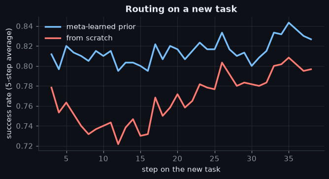
3. A new task: meta-learned prior against learning from scratch#
def curves(prior_mean, prior_n, runs=120, steps=40):
    out = []
    for i in range(runs):
        task = RoutingTask.sample(np.random.default_rng(1000 + i))
        gate = MetaCalibratedGate(task.modules(), prior_mean, prior_n, seed=i)
        out.append(simulate_routing(gate, task, steps, np.random.default_rng(2000 + i))['success'])
    return np.array(out, float)

meta = curves(prior_mean, prior_n)
scratch = curves(np.zeros(4), 1.0)
print('success over the first 25 steps: meta-learned %.3f, from scratch %.3f' % (meta[:, :25].mean(), scratch[:, :25].mean()))
success over the first 25 steps: meta-learned 0.810, from scratch 0.756
def smooth(x, w=5):
    return np.convolve(x, np.ones(w) / w, mode='valid')
fig, ax = plt.subplots(figsize=(6.8, 3.2))
for name, M, c in (('meta-learned prior', meta, theme['palette'][1]), ('from scratch', scratch, theme['palette'][0])):
    m = smooth(M.mean(0))
    ax.plot(np.arange(len(m)) + 3, m, color=c, lw=2.2, label=name)
ax.set_xlabel('step on the new task'); ax.set_ylabel('success rate (5-step average)')
ax.set_title('Routing on a new task'); ax.legend()
plt.show()
The statements below are checked by this cell every time the documentation is built:
early = meta[:, :10].mean() - scratch[:, :10].mean()
late = meta[:, -10:].mean() - scratch[:, -10:].mean()
assert meta[:, :25].mean() > scratch[:, :25].mean() and early > late
print('checked')
checked
The advantage is largest at the start of a task and shrinks as both gates collect task-specific data.
References: Efron & Morris (1975), JASA 70, 311-319 (empirical Bayes); Finn et al. (2017), ICML (meta-learning).