
Calibrated confidence and conformal sets#
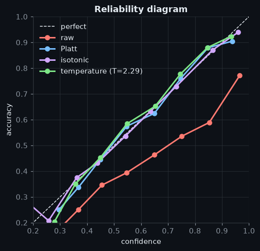
A detector that says “cup, 0.95” is only useful if it is right about 95% of the time when it says so. Deep networks are often over-confident. This tutorial measures calibration with a reliability diagram and the expected calibration error (ECE), fixes it with three recalibration methods, turns scores into conformal prediction sets with a coverage guarantee, and monitors calibration online with an exact confidence bound.
The detector outputs here are simulated with a known amount of over-confidence.
import numpy as np
import matplotlib.pyplot as plt
from quantum_mind.viz import use_mpl_style
from quantum_mind.applications.calibration import (reliability_curve, expected_calibration_error, brier_score,
                                                   PlattScaling, TemperatureScaling, IsotonicCalibration,
                                                   SplitConformalClassifier, CalibrationMonitor, clopper_pearson)
theme = use_mpl_style('dark')
rng = np.random.default_rng(0)

# a 5-class "detector": true class probabilities, then sharpened to make it over-confident
logits = rng.normal(size=(6000, 5)) * 1.6
P_true = np.exp(logits) / np.exp(logits).sum(1, keepdims=True)
y = np.array([rng.choice(5, p=p) for p in P_true])
P_det = P_true ** 2.2 / (P_true ** 2.2).sum(1, keepdims=True)
conf, pred = P_det.max(1), P_det.argmax(1)
correct = pred == y
print('accuracy %.3f   mean confidence %.3f   ECE %.3f' % (correct.mean(), conf.mean(), expected_calibration_error(conf, correct)))
accuracy 0.583 mean confidence 0.778 ECE 0.194
1. Recalibrate on held-out data#
Fit each method on the first half, evaluate on the second.
tr, te = slice(0, 3000), slice(3000, None)
methods = {
    'raw': conf[te],
    'Platt': PlattScaling().fit(conf[tr], correct[tr]).transform(conf[te]),
    'isotonic': IsotonicCalibration().fit(conf[tr], correct[tr]).transform(conf[te]),
}
ts = TemperatureScaling().fit(P_det[tr], y[tr])
methods['temperature (T=%.2f)' % ts.T] = ts.transform(P_det[te]).max(1)
for k, c in methods.items():
    print('%-22s ECE %.3f   Brier %.3f' % (k, expected_calibration_error(c, correct[te]), brier_score(c, correct[te])))
raw                    ECE 0.192   Brier 0.253
Platt                  ECE 0.020   Brier 0.212
isotonic               ECE 0.009   Brier 0.212
temperature (T=2.29)   ECE 0.017   Brier 0.211
fig, ax = plt.subplots(figsize=(5.2, 5.0))
ax.plot([0, 1], [0, 1], color=theme['text'], ls='--', lw=1, label='perfect')
for (k, c), col in zip(methods.items(), theme['palette']):
    r = reliability_curve(c, correct[te], bins=10)
    ok = r['count'] > 0
    ax.plot(r['confidence'][ok], r['accuracy'][ok], 'o-', color=col, lw=2, label=k)
ax.set_xlabel('confidence'); ax.set_ylabel('accuracy'); ax.set_title('Reliability diagram')
ax.legend(loc='upper left'); ax.set_xlim(0.2, 1); ax.set_ylim(0.2, 1)
plt.show()
2. Conformal prediction sets#
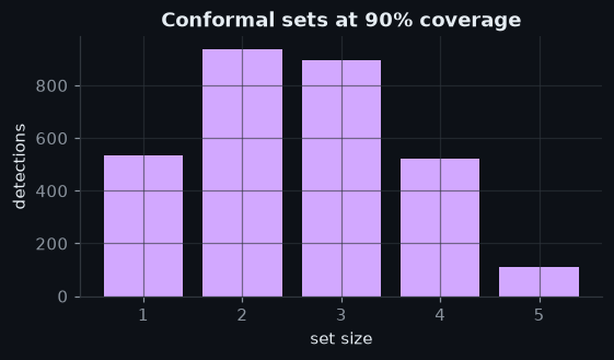
Instead of one label, return the smallest set of labels that contains the truth with probability at least \(1 - \alpha\), guaranteed for exchangeable data. When the set has more than one label, the robot should ask.
for alpha in (0.05, 0.1, 0.2):
    cp = SplitConformalClassifier(alpha=alpha).fit(P_det[tr], y[tr])
    S = cp.predict_sets(P_det[te])
    cover = S[np.arange(S.shape[0]), y[te]].mean()
    print('alpha %.2f: coverage %.3f (target %.2f)   mean set size %.2f   ask rate %.2f'
          % (alpha, cover, 1 - alpha, S.sum(1).mean(), (S.sum(1) > 1).mean()))
alpha 0.05: coverage 0.966 (target 0.95)   mean set size 3.29   ask rate 0.93
alpha 0.10: coverage 0.911 (target 0.90)   mean set size 2.58   ask rate 0.82
alpha 0.20: coverage 0.817 (target 0.80)   mean set size 1.89   ask rate 0.62
cp = SplitConformalClassifier(alpha=0.1).fit(P_det[tr], y[tr])
sizes = cp.predict_sets(P_det[te]).sum(1)
fig, ax = plt.subplots(figsize=(5.6, 2.8))
ax.hist(sizes, bins=np.arange(0.5, 6), rwidth=0.8, color=theme['palette'][2])
ax.set_xlabel('set size'); ax.set_ylabel('detections'); ax.set_title('Conformal sets at 90% coverage')
plt.show()
3. Monitor calibration online#
On the robot, keep counting. CalibrationMonitor tracks accuracy per confidence bin and gives a
Clopper-Pearson lower bound, which risk_aware_ask_or_act can use as p_lower.
mon = CalibrationMonitor(min_count=20)
for c, ok in zip(conf[te], correct[te]):
    mon.update(c, ok)
est, lower = mon.estimate(0.95)
print('when the detector says 0.95: observed accuracy %.3f, 95%% lower bound %.3f' % (est, lower))
print('Clopper-Pearson for 18 of 20 correct:', np.round(clopper_pearson(18, 20), 3))
when the detector says 0.95: observed accuracy 0.771, 95% lower bound 0.745
Clopper-Pearson for 18 of 20 correct: [0.683 0.988]
The statements below are checked by this cell every time the documentation is built:
raw_ece = expected_calibration_error(conf[te], correct[te])
assert all(expected_calibration_error(c, correct[te]) < raw_ece / 2 for k, c in methods.items() if k != 'raw')
S = SplitConformalClassifier(alpha=0.1).fit(P_det[tr], y[tr]).predict_sets(P_det[te])
assert S[np.arange(S.shape[0]), y[te]].mean() >= 0.87          # about 90% coverage, as guaranteed
print('checked')
checked
Summary. Every recalibration method at least halves the calibration error of the over-confident detector, and the conformal sets reach their coverage target.
References: Guo et al. (2017), ICML; Platt (1999); Zadrozny & Elkan (2002), KDD; Angelopoulos & Bates (2023), Foundations and Trends in Machine Learning 16, 494-591; Clopper & Pearson (1934), Biometrika 26, 404-413.