
Bistable perception and the quantum Zeno effect#
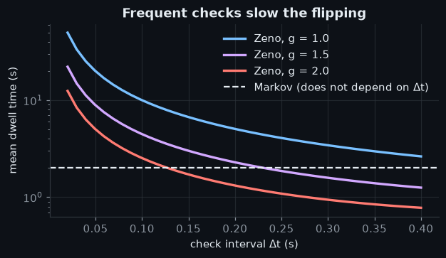
Look at a Necker cube and your perception flips between two 3D interpretations. How long each interpretation lasts (its dwell time) has been measured in many experiments. The quantum Zeno model treats the percept as a two-state system that slowly rotates from one interpretation to the other, while the brain “checks” the percept every \(\Delta t\); each check projects it back. Frequent checks slow the flipping (the Zeno effect), so the model predicts a mean dwell time of about \(\Delta t / \sin^2(g\,\Delta t)\), which grows as \(1/\Delta t\) when checks are frequent.
This tutorial compares the Zeno model with two classical baselines, a Markov switching model (constant flip rate) and a gamma renewal model (the usual descriptive fit), on simulated dwell times.
import numpy as np
import matplotlib.pyplot as plt
from quantum_mind.viz import use_mpl_style
from quantum_mind.core import compare
from quantum_mind.families.perception import (QuantumZenoBistableModel, MarkovSwitchingModel, GammaRenewalModel,
                                              dwell_time_design, mean_dwell_time)
theme = use_mpl_style('dark')
zeno = QuantumZenoBistableModel(g=1.5)
1. The Zeno signature: dwell time against check interval#
dts = np.linspace(0.02, 0.4, 40)
fig, ax = plt.subplots(figsize=(6.4, 3.2))
for g, c in ((1.0, theme['palette'][1]), (1.5, theme['palette'][2]), (2.0, theme['palette'][0])):
    ax.plot(dts, [mean_dwell_time(QuantumZenoBistableModel(g=g), dt) for dt in dts], color=c, lw=2.2, label='Zeno, g = %.1f' % g)
ax.axhline(MarkovSwitchingModel(rate=0.5).mean_dwell(0.1), color=theme['text'], ls='--', label='Markov (does not depend on Δt)')
ax.set_xlabel('check interval Δt (s)'); ax.set_ylabel('mean dwell time (s)'); ax.set_yscale('log')
ax.set_title('Frequent checks slow the flipping'); ax.legend()
plt.show()
2. Dwell-time distributions#
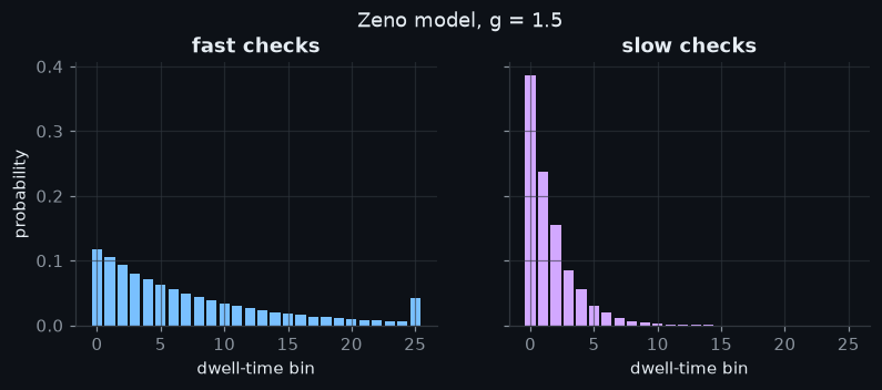
design = dwell_time_design({'fast checks': 0.035, 'slow checks': 0.14}, max_time=40, n_bins=25)
pred = zeno.predict(design)
fig, axes = plt.subplots(1, 2, figsize=(8.4, 2.8), sharey=True)
for ax, (cond, p), c in zip(axes, pred.items(), theme['palette'][1:]):
    ax.bar(range(len(p)), p, color=c); ax.set_title(cond); ax.set_xlabel('dwell-time bin')
axes[0].set_ylabel('probability'); fig.suptitle('Zeno model, g = 1.5', y=1.03)
plt.show()
3. Can the data tell the models apart?#
With one check interval, the models can mimic each other. With two intervals the Zeno model’s specific scaling identifies it.
ranking = {}
for name, conds in (('one interval', {'only': 0.07}), ('two intervals', {'fast': 0.035, 'slow': 0.14})):
    d = dwell_time_design(conds, max_time=40, n_bins=25)
    data = zeno.sample(d, 300, np.random.default_rng(0))
    res = compare([QuantumZenoBistableModel, MarkovSwitchingModel, GammaRenewalModel], data, d)
    ranking[name] = {type(r.model).__name__: r.bic for r in res}
    print('%-14s ' % name + '   '.join('%s BIC %.1f' % (type(r.model).__name__.replace('Model', ''), r.bic) for r in res))
one interval QuantumZenoBistable BIC 1428.9 MarkovSwitching BIC 1429.3 GammaRenewal BIC 1433.9
two intervals QuantumZenoBistable BIC 2796.6 GammaRenewal BIC 3031.8 MarkovSwitching BIC 3073.8
The statements below are checked by this cell every time the documentation is built:
one, two = ranking['one interval'], ranking['two intervals']
assert abs(one['QuantumZenoBistableModel'] - one['MarkovSwitchingModel']) < 10     # one interval: hard to tell apart
assert min(two, key=two.get) == 'QuantumZenoBistableModel' and min(v for k, v in two.items() if k != 'QuantumZenoBistableModel') - two['QuantumZenoBistableModel'] > 10
print('checked')
checked
Summary. The Zeno model makes a testable prediction (dwell time against check interval) that the baselines do not; an experiment needs at least two observation rates to test it.
References: Atmanspacher, Filk & Römer (2004), Biological Cybernetics 90, 33-40; Atmanspacher & Filk (2010), Journal of Mathematical Psychology 54, 314-321; Brascamp et al. (2006), Journal of Vision 6, 1244-1256.